


Россия
BISAC NAT010000 Ecology
BISAC NAT045050 Ecosystems & Habitats / Coastal Regions & Shorelines
BISAC NAT025000 Ecosystems & Habitats / Oceans & Seas
BISAC NAT045030 Ecosystems & Habitats / Polar Regions
BISAC SCI081000 Earth Sciences / Hydrology
BISAC SCI092000 Global Warming & Climate Change
BISAC SCI020000 Life Sciences / Ecology
BISAC SCI039000 Life Sciences / Marine Biology
BISAC SOC053000 Regional Studies
BISAC TEC060000 Marine & Naval
In this study, a three-dimensional numerical model for cold water jets in the coastal region is developed for the calculation of not only the initial mixing but also horizontal dispersion above the seabed. The computed velocities and temperatures were compared with the measurements obtained in the scaled hydraulic experiment. The good agreement with measurements confirms the model provides appropriate results for cold water dispersion. Our numerical results indicate that coastal topography is the most important factor in determining areas influenced by discharged cold water.
negative buoyant jet, density current, k-ε model, LNG plant
- INTRODUCTION
Water jets discharged into an ocean are of significant interest in coastal environmental management [1, 2, and 3]. When the discharged water is denser than the ambient water, it drops to the bottom of the ocean and forms a density current. Well-known examples of such negatively buoyant jets are cold water released from liquefied natural gas (LNG) plants and brine released from desalinization plants. This phenomenon may affect local benthic communities [4, 5]. It is essential to develop an appropriate numerical model for the transport and mixing behavior of the negatively buoyant jets in coastal areas for assessing the potential impacts of discharged cold water on the coastal environment.
When studying the dispersions of negatively buoyant jets in the coastal area, two regions with different behavior should be considered: the near fields and the far field. The near field region is located in the vicinity of outlets and is characterized by the initial mixing, depending on the discharge configuration design. The far field region is located further away from the outlets, where the stream forms into density current that flows down along the seabed, depending the coastal topography and tidal currents.
There has been some numerical study on negatively buoyant jets. Most of the previous study focused on the initial mixing process and used integral models such as CORMIX, VISUAL PLUMES, and VISJET [6, 7]. However, reference [7] reported significant discrepancies in the dilution predictions by these integral models for the negatively buoyant jet modeling. Reference [8] computed initial mixing of brine jets using the software CFX with k-e model and pointed out that the k-e model provided a more accurate representation of the initial mixing process compared to the integral model. Recently, reference [9] reported large eddy simulation for the initial mixing of the brine jets using the open source code OpenFOAM.
For the positive buoyant jet such as thermal water discharged from power plants, reference [2] calculates the initial mixing at near field and density current in far fields. For the negatively buoyant jets, however, because of limited spatial coverage in experiments and the lack of a robust numerical modeling approach, the downstream concentration fields beyond the initial dilution zone, which are affected by complicated coastal topography, are largely unknown.
In this study, a three-dimensional k-ε model for cold water jets in the coastal region is developed for the calculation of not only the initial mixing but also horizontal dispersion above the seabed. The fractional-area-volume-obstacle-representation (FAVOR) method [10] was employed for computing flows bounded by complicated geometric shapes. The computed velocities and temperatures were compared with the measured values obtained in the scaled hydraulic experiments.
This paper is organized as follows. Section II interprets our numerical model. Section III explains the numerical conditions. Section IV describes the numerical results. Finally, Section V states the summary.
- Numerical model
In this study, we solved the Reynolds-averaged Navier-Stokes (RANS) equations using the heat transport equation. The Reynolds-averaged equations of mass and momentum can be expressed as
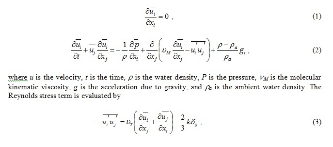
where nT is the coefficient of eddy viscosity, k is the turbulent energy, and dij is the Kronecker delta. We used the k-e model to estimate the eddy viscosity. In this model, nT is parameterized by the turbulent energy k and energy dissipation rate e. However, in stably stratified environments, the turbulent motions in the vertical direction are impeded by the buoyancy forces [11]. Thus, the eddy viscosity should be separated into horizontal eddy viscosity and vertical eddy viscosity. In this study, we compute the horizontal and vertical eddy viscosities using the following equations [12].
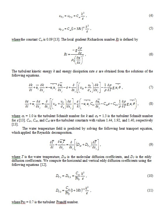
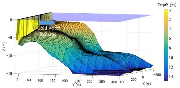
Fig. 1. Coastal topography
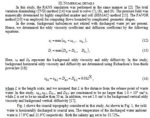
Table 1. Numerical conditions
|
Case |
Outlet type |
Cold water flow rate (m3/s) |
Outlet velocity (m/s) |
Outlet depth (m) |
Computational grids (x, y, z) |
|
1 |
Pipes (f 1.3 m × 2) |
4.6 |
1.73 |
-2.05 |
90 × 50 × 48 |
|
2 |
Multiport diffuser (f 0.72 m × 5) |
4.1 |
2.01 |
-2.9 |
92 × 79 × 44 |
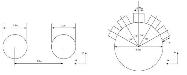
Fig. 2. Schematic of wastewater outlets in case 1 (left) and case 2 (right).
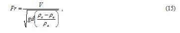
Two different computations were performed, as shown in Table 1. In case1, the cold water is discharged from two pipes (Fig. 2a). In case2, the cold water is discharged from a multiport diffuser (Fig. 2b). A computational mesh in the Cartesian coordinate system (x, y, z) was used in the box-shaped domain. Fig. 3 shows the computational mesh used in case 1. We used a non-uniform computational grid to reduce the computational cost.
To validate the model, the computed velocities and temperatures were compared with the experiments in the scaled hydraulic model [18]. The hydraulic model was not geometrically distorted and the geometric length scale ratio was 1/50. The flow was scaled according to the similarity of Froude criterion [18]. We maintained the same value of the densimetric Froude number Fr between the model and prototype. The densimetric Froude number Fr is
where V is the water discharge velocity, d is the pipe diameter, and rc is the density of the discharged water.
- RESULTS AND DISCUSSIONS
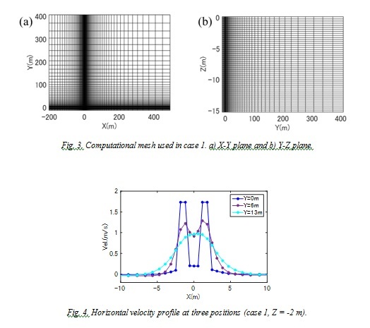
The initial mixing process is an important process that affects the diffusion of cold water. Fig. 4 shows the horizontal velocity profile at three positions (Y = 0, 6, 13 m) in case1. The distribution width increased with increasing distance because the turbulent jets entrain the ambient water. The entrainment phenomenon creates a depressurized region between two jets. The location of maximum velocity can be defined as the jet centerline. The jets discharged from the nearby-submerged two pipes generate complex trajectories. The depressurized region causes deflection of the jet trajectories [19]. Finally, they are merged and behave like a single jet.
Fig. 5 shows the decay of the maximum velocity in Y direction. The computational values were compared to the measured values in the scaled hydraulic model to validate
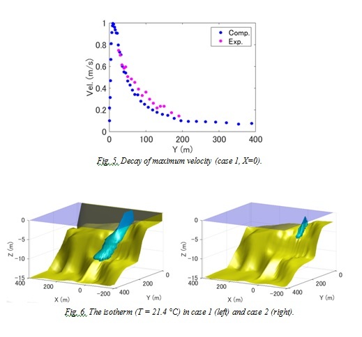
our model quantitatively. After the merge point (Y = 13 m), both the computational and experimental velocities indicate exponential decay, and computational results agree well with experimental results.
The momentum decay of the jet causes descent of the jet due to the negative buoyancy. Fig. 6 shows the isotherm of the water temperature. After the jet reaches the bottom of the ocean, the stream flows along the seabed as a gravity-driven density current that entrains the ambient water gradually. Hence, the seabed morphology is a primary factor in determining the area affected by the discharged cold water.
While the flow rates in case 1 and case 2 are nearly equal, the isotherm in case 2 is dramatically narrow compared to the one in case1. Fig. 7 shows the horizontal distributions of the minimum temperature at the center plane in case 1 and case 2. The water temperature in the vicinity of the outlets is reduced drastically. The water temperature increases with increasing distance from the outlet. The water temperature in case 2 reaches 21.4°C at Y = 100m, while the temperature in case1 reaches 21.4°C at Y = 260 m. This is because the difference in the outlet velocity of both cases
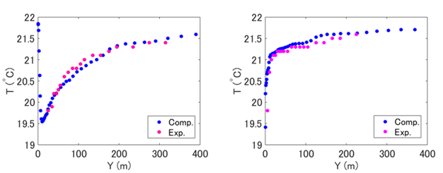
Fig. 7. Spanwise variation of minimum temperature in the X = 0 plane in case 1 (left) and case 2 (right).
(Table 1). The high outlet velocity in case 2 causes the enhancement of entrainment, which results in the rapid mixing of the discharged water with the ambient water.
Fig. 7 also shows the measured temperatures in the scaled hydraulic model to compare with the computational results. It is found that the computed temperature is consistent with the measured decrease in temperature. Agreements with experimental results confirm that the model appropriately evaluates the dispersion of the cold water discharged from both the pipe and multiport diffuser.
- CONCLUSION
In this study, a three-dimensional k-ε model for negative buoyant jets in the coastal zone is developed. The model can calculate the flow along the seabed using the FAVOR method.
The proposed model reproduced the mixing and diffusion processes of a cold water jet. The computed velocities and temperatures were compared with the measured values obtained in the scaled hydraulic model. The results showed good agreement with each other for both fluid velocity and temperature, demonstrating that the model appropriately evaluates the dispersion of the discharged cold water. Our numerical results indicate that coastal topography is the most important factor in determining areas affected by the discharged cold water.
- ACKNOWLEDGMENT
The authors thank S. Nagoya and I. Okawa for their help in performing computations and experiments.
1. H.B. Fischer, E.J. List, R.C.Y. Koh, J. Imberger, and N.H. Brooks, Mixing in Inland and Coastal Waters. Academic Press, 1979.
2. T. Tsubono, S. Sakai, S. Matsunashi, M. Mizutori, “Mixing Process of Heated Water Adjacently Discharged from Surface and Submerged Outlets-Improvement and Verification of a 3-D Numerical Simulation Model - (in Japanese)”, CRIEPI Research Report, U00013, 2000.
3. T. Yanagi, K. Sugimatsu, H. Shibaki, H.-R. Shin, and H.-S. Kim, “Effect of tidal flat on the thermal effluent dispersion from a power plant,” J. Geophys. Res., vol. 110, C03025, 2005.
4. M. Milione and C. Zeng, “The effects of temperature and salinity on population growth and egg hatching success of the tropical calanoid copepod, Acartia sinjiensis,” Aquaculture, 275, 116-123, 2008.
5. D. Drami, Y.Z. Yacobi, N. Stambler, and N. Kress, “Seawater quality and microbial communities at a desalination plant marine outfall. A field study at the Israeli Mediterranean coast,” Water Research, 45, 5449-5462, 2011.
6. P. Palomar, J.L. Lara, I.J. Losada, M. Rodrigo and A. Alvarez, “Near field brine discharge modelling part 1: Analysis of commercial tools,” Desalination, 290, 14-27, 2012.
7. P. Palomar, J.L. Lara, and I.J. Losada, “Near field brine discharge modelling part 2: Validation of commercial tools,” Desalination, 290, 28-42, 2012.
8. C.J. Oliver, M.J. Davidson, and R.I. Nokes, “k- Predictions of the initial mixing of desalination discharges,” Environmental Fluid Mechanics, 8, 617-625, 2008.
9. S. Zhang, B. Jiang, A.W.-K. Law, and B. Zhao, “Large eddy simulations of 45° inclined dense jets,” Environmental Fluid Mechanics, 16, 101-121, 2016.
10. C.W. Hirt and J.M Sicilian, “A porosity technique for the definition of obstacles in rectangular cell meshes,” International Conference on Numerical Ship Hydrodynamics, 1985.
11. P. Huq, and D.D. Stretch, “Critical dissipation rates in density stratified turbulence,” Physics of Fluids, Vol. 7, No. 5, pp. 1034-1039, 1995.
12. S. Bloss, R. Lehfeldt and J.C. Patterson, “Modeling turbulent transport in stratified estuary,” Journal of Hydraulic Engineering, Vol. 114, No. 9, pp. 1115-1133, 1988.
13. S.B. Pope, Turbulent Flows. Cambridge University Press, 2000.
14. P.L. Roe, “Approximate Riemann solvers, parameter vectors, and different schemes,” Journal of Computational Physics, 43, 357-372, 1981.
15. C.W. Hirt and J.L Cook, “Calculating three-dimensional flows around structures and over rough terrain,” Journal of Computational Physics, Vol. 10, pp. 324-340, 1972.
16. A. Okubo, “Some speculations on oceanic diffusion diagrams,” Rapport des Proces-Verbaux des Reunions du Conseil International pour l’Exploration de la Mer, 167, pp. 77-85, 1974.
17. S.A. Thrope, The Turbulent Ocean. Cambridge University Press, 2005.
18. S.A. Hughes, Physical Models and Laboratory Techniques in Coastal Engineering. World Scientific, 1993.
19. E. Tanaka, “The interference of two-dimensional parallel jets,” Bulletin of the JSME, Vol. 17, No.109, pp. 920-927, 1974.