


BISAC NAT010000 Ecology
BISAC NAT045050 Ecosystems & Habitats / Coastal Regions & Shorelines
BISAC NAT025000 Ecosystems & Habitats / Oceans & Seas
BISAC NAT045030 Ecosystems & Habitats / Polar Regions
BISAC SCI081000 Earth Sciences / Hydrology
BISAC SCI092000 Global Warming & Climate Change
BISAC SCI020000 Life Sciences / Ecology
BISAC SCI039000 Life Sciences / Marine Biology
BISAC SOC053000 Regional Studies
BISAC TEC060000 Marine & Naval
In order to understand the temporal variation of the physics and fluid structure of Yodo River estuary in detail, we had made in-situ observation. And the temporal variation of Alexandrium tamarense which cause the shellfish poisoning of natural freshwater clam was analyzed by the numerical ecosystem model which is considered the salinity effects. Stratification develops in the downstream side. Chl.a concentration is high in the seawater region. A. tamarense is detected in the downstream side. The numerical ecosystem model including the salinity effect for A. tamarense was formulated. A. tamarense grow only in the bottom layer in daytime, and the daily mean of it is 7 % of it transported from Osaka Bay. A. tamarense is transported to the upstream in flood tide. 81 % of it transported from Osaka Bay goes to the upstream zone. Much A. tamarense transported to the upstream zone in nighttime due to the vertical migration. Therefore when it is the flood tide in nighttime, more of A. tamarense might be transported to the upstream zone.
Alexandrium tamarense, Yodo River, estuary, numerical ecosystem model, red tide, shellfish poisoning
I. Introduction
The Yodo River estuary shown in Fig. 1 which is defined in this research as a zone from the river mouth up to 10 km, has fisheries of natural freshwater clam around at 5 km from the river mouth. Shellfish poisoning of natural freshwater clam occurred intermittently in the estuary in spring since 2007, and the shipment of freshwater clams was halted due to government regulations. Cause of the shellfish poison is Alexandrium tamarense [1] which is poisonous marine phytoplankton appearing in Osaka Bay every year, and can growth in salinity environment of more than 15 [2]. The lack of fresh water discharge from the weir promoted the initiation of the bloom of A. tamarense [3]. In order to understand the temporal variation of the physics and fluid structure of the area in detail, we made in-situ observation and analyzed the temporal variation of A. tamarense by using the numerical ecosystem model.
II. Methods
The observation was carried out during April 2nd and 3rd in 2012 in the neap tide. Vertical profiles of water temperature (T), salinity (S), fluorescence, photon (I) and so on were measured by CTD (the conductivity, temperature and depth profiler) in 10 cm width at 5 stations in the intertidal zone between the river mouth and the Yodo River weir shown in Fig. 1. Surface water (0 m) and the bottom water which is above 1 m from the bottom were sampled at the same time by a bucket and Kitahara water sampler, respectively. Sampled water was dispensed to the poly bottles, and was analyzed for the chemical and biological analysis. The items are cell density of A. tamarense, Chl.a (chlorophyll-a), TP (total phosphorus) and DIP (dissolved inorganic phosphorous) concentrations and so on. Sampled water were kept in the dark and cool condition, and were transported to Research Institute of Environment, Agriculture and Fisheries, Osaka Prefecture to count the cell density, and to Hyogo Environmental Advancement Association to analyze Chl.a, TP and DIP concentrations and so on. The fluorescence values of CTD were converted into Chl.a concentrations using the analyzed Chl.a concentrations. ADCP (Acoustic Doppler Current Profiler) observation was carried out along the traverse line (L1 in Fig. 1) at the river mouth in every 23 cm depth at 0.2 Hz. The observation was repeated 4 cycles during one tidal period shown in Fig. 2(a). The water level was monitored every 10 minutes at Fukushima as shown in Fig. 1 by the Yodogawa River Office, Kinki Regional Development Bureau, Ministry of Land, Infrastructure and Transport.
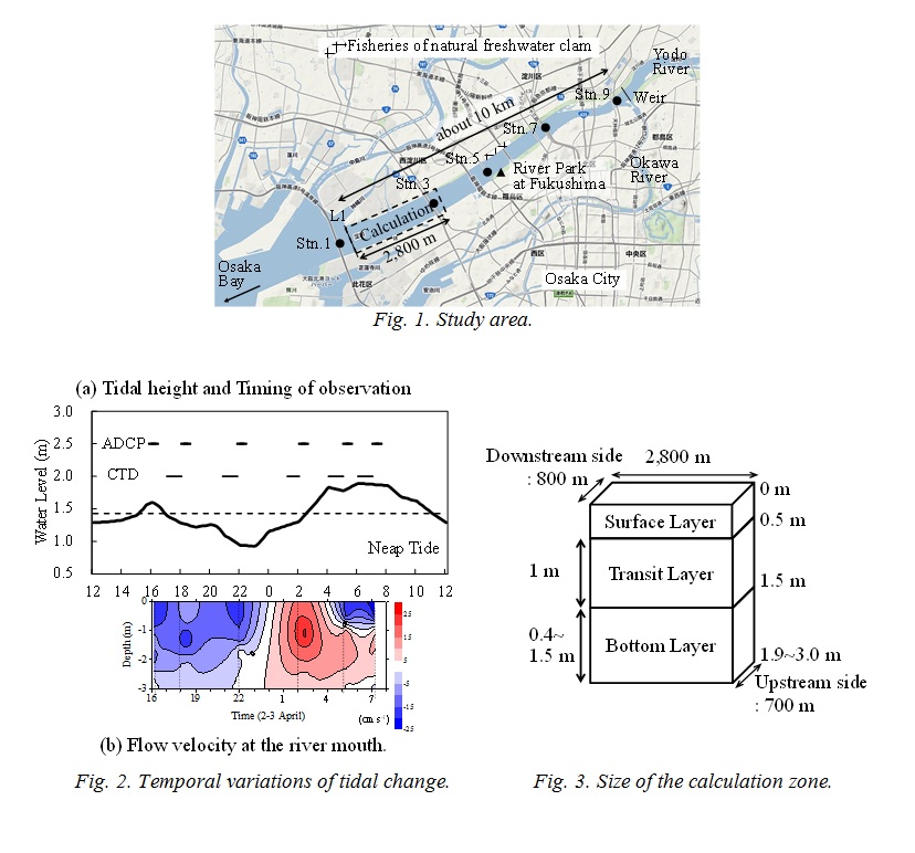
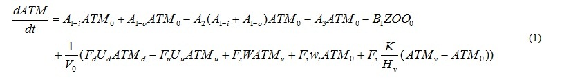
The calculation zone by the numerical ecosystem model shown in Fig. 1 is from L1 up to 2,800 m upstream. Water depth became deeper toward the upstream side, and is shallow in the outside of the upstream boundary. Stn. 3 is included in the zone. The calculation zone was divided into the surface layer (above 0.5 m), the transition layer (0.5-1.5 m) and the bottom layer (below 1.5 m) as shown in Fig. 3. The phosphorus (P) cycling during 24 hours, which is one tidal period of the day was calculated. DIN/DIP ratio is larger than the Redfield ratio (C:N:P=106:16:1) in this observation. It means that the primary production is limited by DIP. The compartments of the numerical ecosystem model is shown in Fig. 4. The types of P are DIP, DOP, phytoplankton, A. tamarense, zooplankton and detritus, and are changed by the biochemical processes. Phytoplankton in this research means other than A. tamarense, and is mainly diatom. A. tamarense utilizes DOP in photosynthesis. The exchange processes between the layers or the outside of the area are the horizontal and vertical advection, the vertical diffusion, the natural sinking of phytoplankton and detritus and the diurnal vertical migration of A. tamarense. A. tamarense move to the surface during the day, and move to the bottom during the night. The horizontal diffusion would be quite small compere to the horizontal advection. Therefore the horizontal diffusion is not assumed. The water depth is shallow in the river. So, the vertical advection speed is assumed as a constant in each depth. The upstream and upward fluxes are positive.
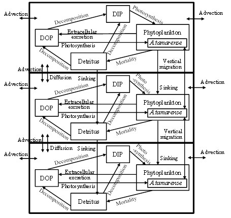
Fig. 4. The compartments of the numerical ecosystem model
Temporal changes in P concentration of each compartment, P in phytoplankton, A. tamarense, zooplankton and detritus, DIP and DOP, are represented by the equations. For example, equation (1) represents the temporal change of P concentration in A. tamarense (ATM). The first and second terms mean photosynthesis. The 3rd term means extra cellular excretion of DOP by photosynthesis. The 4th term means mortality. The 5th term means grazing by zooplankton. The 6th term means the horizontal and vertical transports including the vertical migration.
where A’s are the coefficients of biochemical processes related to phytoplankton, and will be explained later. B1 represents grazing by zooplankton. Subscripts of the concentrations mean place. Subscript 0 refers to the calculating layer. Subscript d and u refer to the downstream and upstream side, respectively. But when the water flows out from the calculation layer, the concentration of the calculated layer should be used. Subscript v refers to the source layer of outflow. V0 is the volume of the calculation layer. Hv is the distance between the surface and transition or the transition and bottom layers. F’s are the section. U’s are the horizontal advection velocity. Subscript d refers to the downstream side, u is the upstream side, and s is the surface. W is the vertical advection speed. K is the vertical eddy diffusivity. The estimation mothed of U, W and K will be explained later. wt is the vertical migration speed of A. tamarense. It is wt>0 during the day (at 06-18), and means the upward motion. It is wt<0 during the night (at 18-06), and means the downward motion. Moreover, A. tamarense would not swim to the lower salinity layer. Therefore, the vertical migration is stopped not to move to the layer that salinity is below the threshold. The terms of vertical advection, diffusion and migration are double in the transition layer which have two boundaries with the upper and lower sides.
A1 represents the photosynthesis, and is the function of DIP or DOP concentration (DIP0, DOP0), T, I and S. Equation (2) shows in case of DIP. A1 of phytoplankton does not include the term of salinity. And phytoplankton does not used DOP in photosynthesis.

The term of nutrient represents by the Michaelis-Menten equation. Vmax is the maximum uptake ratio of nutrient. kp is the half saturation constant of nutrient for phytoplankton. V is Vmax and kp are different depending on the type of nutrients and the phytoplankton spices. Shapes of the temperature and photon terms represent that growth is most active in the optimum water temperature (To) and photon (Io). However photoinhibition do not occur even when the photon in the water is more than Io. So, I=Io is applied when I>Io. The function of salinity effect is formulated based on the result of incubation shown in Fig. 5 [2]. And the threshold of salinity (Sg*) which stop the growth of A. tamarense, and the coefficient of salinity dependency in the photosynthesis of A. tamarense (kgs) are given.
A2 is the coefficient of the extra cellular excretion of DOP by photosynthesis. A3 represents the mortality, and is given by the following equation which is the function of T, and of S only case of A. tamarense. The function of salinity effect is also formulated by Fig. 5.

where mp0 is the mortality speed of phytoplankton at 0 deg-C, km-p is the temperature dependency of mortality for phytoplankton, kms is the salinity dependency of mortality for A. tamarense, Sm* is the threshold of salinity in photosynthesis of A. tamarense. Mortality accelerates when salinity is over Sm*.
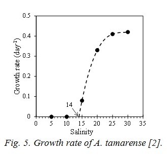
Parameters of constant of the ecosystem model are shown in Table 1, and are referred to the previous study [4]. It analyzed the competitive relationship of diatom and non-diatom in the inner part of Osaka Bay which is the estuary of the Yodo River. wt has been tuned to reproduce the observed value, and is 1/20 of the value by reference [4]. Vmax and kp related to photosynthesis are referred to previous study [5] based on the incubation by using the Yodo River water. The parameters of salinity for A. tamarense were determined based on Fig. 5.
The data sets of the boundary and environmental conditions of T, S, I, V, Hv and Fv, which vary temporally and are inputted to the model every minute for 24 hours, were constructed by the observation data. The variations of salinity are 1.0-2.2 in the surface layer, 9.1-12.7 in the transition layer and 24.6-26.5 in the bottom layer. Salinity in the surface and transition layer are always less than 14 which is the threshold of salinity in photosynthesis of A. tamarense. The variations of water temperature is 10.8-11.6 deg-C which is lower than the optimum water temperature. Photoenvironments were the optimum condition at 6 to 18 in the surface layer and at 8 to 16 in the transition layer. Photon in the bottom layer was 7 % of it in the surface layer, and is enough for photosynthesis.
P concentrations in Stn. 1 were used as the boundary condition of the downstream side, and it in Stn. 5 was used as the upstream side. P concentrations in phytoplankton were calculated by Chl.a concentration converted from fluorescence values of CTD and P/Chl.a which was estimated by C/Chl.a=30 [6], the Redfield ratio and the atomic weight of C and P. P concentrations in zooplankton were assumed 10 % of phytoplankton. P concentrations in A. tamarense estimated by the cell density and P weigh par cell which calculated by C weigh per cell and the Redfield ratio. 2,000 pg-C cell-1 [7] was used, then 48.7 pg-P cell-1 was obtained. TP:DOP in the inter tidal zone of Yodo Rivre is 14.5 % [8]. P concentrations in detritus is obtained by subtracting these concentrations from the TP.
Table 1. Values of the parameter used in the ecosystem model.
III. Results and Discussions
Stratification develops in the downstream side. Seawater intrudes to close to Stn.9 in flood and high tides. And Chl.a concentration is high in the seawater region. Seawater intrusion stops at around Stn.7 in ebb and low tides. High concentration of Chl.a near the surface would be freshwater phytoplankton. Seawater expansion to the river spread a habitat of marine phytoplankton [9]. A. tamarense is detected in the downstream side mainly, therefore the calculation zone has been set at the river mouth. However, the cell density is small, and the red tide was not formulated in this year. Figure 2(b) shows the depth-time cross section of the flow velocity at the river mouth. Plus means the upstream flow. It is the downstream flow in all depth from the observation start until 23 o’clock which is weak ebb tide. It is the upstream flow in all depth from 1 to 4 o’clock which is flood tide. Since the variations of horizontal advection by the budget estimates, it is the downstream flow in all boundaries during 13-21. Therefore, this period was defined as ebb tide. And the other period, during 21-13, was defined as flood tide. The estimated vertical advection velocity is ±9×10⁻³ cm s-1, and the vertical diffusion coefficient is 10-5-10-4 cm s-2.
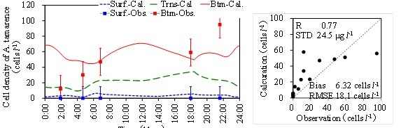
(a) Temporal variations of calculation and observation (b) Correlation with statistical values.
Fig. 6. Calculation result of A. tamarense.
Figure 6(a) is the results of cell density of A. tamarense. Dots show the observed data with the error bar which means the conversion error from concentration in cell density. The results almost reproduced the observed values. Figure 6(b) shows the correlation chart with statistical values. DIP and Chl.a concentrations are under estimate because freshwater phytoplankton is not considered in the model. But A. tamarense is over estimate a little especially in the surface layer. Phytoplankton tends to increase only in the daytime in the bottom layer. Since A. tamarense move to the bottom during night, the increase tendency is also in the nighttime a little.
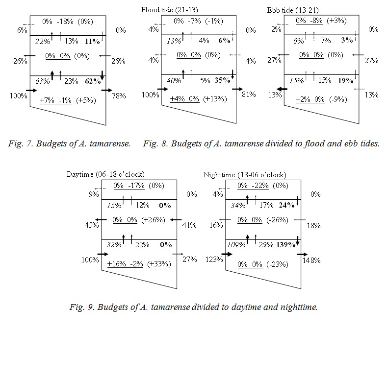
Figure 7 shows the budgets of A. tamarense. Each number is total flux of 24 hours, and has been standardized by the horizontal advection, 4,185×103 mg, to the bottom layer of the downstream boundary. The standard number means the volume of A. tamarense supplied from Osaka Bay. A. tamarense grow only in the bottom layer, and the volume is 7 % of it from Osaka Bay (the numbers at the left side with an underline means photosynthesis in Fig. 8). A. tamarense dies at the surface layer (the numbers at the right side with an underline means mortality & grazing), and moves to the bottom layer by the diurnal migration (the numbers of bold type means diurnal migration). These are salinity effect. 78 % of A. tamarense transported from Osaka Bay to the bottom layer goes to the upstream zone (the numbers without decorations means advection). And 26% returns to the transit layer. 52% of A. tamarense transported from Osaka Bay is lost in the upstream zone. A. tamarense is increased in the bottom layer (the numbers in parentheses mean the budget). It suggests the long term variation, for example, spring and neap tide, and the seasonal variation.
Figure 8 shows the budgets which is divided to flood and ebb tides. Each number has been also standardized, and the volume in flood tide, 4,185×103 mg, was used in this case. A. tamarense is transported from Osaka Bay to the upstream zone in flood tide mainly (81%), and the half of this is returned in ebb tide (27+13 %). Other half is lost in the upstream zone. Return volume to the transit layer is larger than to the bottom layer. A. tamarense would not go to lower salinity layer by itself. So, it is considered that A. tamarense will be transported by the vertical advection and/or diffusion. Figure 9 shows the budgets which is divided to the daytime and nighttime. Each number has been also standardized, and the volume in daytime, 1,878×103 mg, was used in this case. A. tamarense grow only in daytime in the bottom layer, and the volume is 16 % of it from Osaka Bay. A. tamarense do not go to the transit and the surface layers by itself even daytime because of low salinity, but is transported by the vertical advection (12+22 %) and diffusion (15+32 %). Therefore A. tamarense died at the surface layer (17 % & 22 %), and transported not so much to the upstream zone (27 %). A. tamarense is also transported by the vertical advection (17+29 %) and diffusion (34+109 %) in nighttime. However the comparable volume (24 % & 139 %) move to the bottom layer by itself. Therefore much A. tamarense (148 %) transported from the ocean go through upstream.
IV. Conclusion
In order to understand the temporal variation of the physics and fluid structure of Yodo River estuary in detail, we had made in-situ observation. And the temporal variation of A. tamarense which cause the shellfish poisoning of natural freshwater clam was analyzed by the numerical ecosystem model which is considered the salinity effects.
Stratification develops in the downstream side. Chl.a concentration is high in the seawater region. A. tamarense is detected in the downstream side. The numerical ecosystem model including the salinity effect for A. tamarense was formulated. A. tamarense grow only in the bottom layer in daytime, and the daily mean of it is 7 % of it transported from Osaka Bay. A. tamarense is transported to the upstream in flood tide. 81 % of it transported from Osaka Bay goes to the upstream zone. Much A. tamarense transported to the upstream zone in nighttime due to the vertical migration. Therefore when it is the flood tide in nighttime, more of A. tamarense might be transported to the upstream zone.
V. Acknowledgment
This research is supported by Osaka Bay Regional Office Environmental Improvement Center, Dr. Koigo Yamamoto, Research Institute of Environment, Agriculture and Fisheries, Osaka Prefecture, Dr. Tomoyasu Fujii, Nara University of Education, Mr. Nobuo Nozaki, Dr. Kohei Hirono, Mr. Ippei Nakamura and Dr. Satoshi Nakada, Kobe University, the Yodogawa River Office, Kinki Regional Development Bureau, Ministry of Land, Infrastructure and Transport, Waterfront Vitalization and Environment Research Foundation, Dr. Takeshi Matsuno and Dr. Daisuke Ishii, Kyushu University.
1. K. Yamamoto, H. Homi, and M. Sano, “Occurrence of a red tide of the toxic dinoflagellate Alexsandrium tamarense in the estuary of the Yodo River in 2007 -Dynamics of the vegetative cells and the cysts,” Bull. Plankton Soc. Japan, vol. 58(2), pp. 136-145, 2011(in Japanese).
2. P. Lim, and T. Ogata, “Salinity effect on growth and toxin production of four tropical Alexandrium species (Dinophyceae),” Toxicon, vol. 45, pp. 699-710, 2005.
3. K. Yamamoto, H. Tsujimura, M. Nakajima, and P. J. Harrison, “Flushing rate and salinity may control the blooms of the toxic dinoflagellate Alexandrium tamarense in a river/estuary in Osaka Bay, Japan,” J. Oceanogr. vol. 69, pp. 727-736, 2013.
4. M. Hayashi, and T. Yanagi, “Analysis of change of red tide species in Yodo River estuary by the numerical ecosystem model,” Marine Pollution Bulletin, vol. 57, pp. 103-107, 2008.
5. M. Natsuike, I. Imai, K. Yamamoto, and M. Nakajima, “Effects of phosphorus supply from the Yodo River water on interspecific competition between Alexandrium tamarense and Skeletonema sp.,” Setonaikai, vol. 66, pp. 50-53, 2013 (in Japanese).
6. T.R. Parsons, Y. Maita, and C.M. Lalli, A Manual of Chemical and Biological Methods for Seawater Analysis, Pergamon Press, Oxford, 1984, pp. 173.
7. T. Yamamoto, “Phytoplankton,” in Marine Coastal Environment, T. Hirano, Eds. Tokyo, Fuji techno-system, 1998, pp. 144-174 (in Japanese).
8. Y. Nakaguchi, Y. Yamaguchi, T. Nishimura,Y. Hatano, M. Imanaka, and Y. Arii, “Behavior and seasonal variation of eutrophication substances in the Yodo River system,” Chikyukagaku (Geochemistry), vol. 39, pp. 173-182, 2005 (in Japanese).
9. M. Hayashi, R. Koga, T. Fujii, and K, Yamamoto, “Analysis of Seawater Run Up in the Yodo River Estuary,” Proc. EMECS 10- MEDCOAST 2013 Joint Conference, vol. 2, pp. 1225-1235, August 2013.