


BISAC NAT010000 Ecology
BISAC NAT045050 Ecosystems & Habitats / Coastal Regions & Shorelines
BISAC NAT025000 Ecosystems & Habitats / Oceans & Seas
BISAC NAT045030 Ecosystems & Habitats / Polar Regions
BISAC SCI081000 Earth Sciences / Hydrology
BISAC SCI092000 Global Warming & Climate Change
BISAC SCI020000 Life Sciences / Ecology
BISAC SCI039000 Life Sciences / Marine Biology
BISAC SOC053000 Regional Studies
BISAC TEC060000 Marine & Naval
A numerical experiment on reconstruction of currents was conducted with real atmospheric forcing data in autumn period of 2007 on the basis of Marine hydrophysical institute (MHI) hydrodynamic model, which was adapted to the coastal area of the Black Sea with an open boundary (north-western shelf). A high resolution (horizontal grid 500500 m and 44 verti-cal layers from 1 m to 49 m) and detailed bathymetry with resolution ~1.6 km were used in the calculation. A higher spatial resolution allowed to get a detailed mesoscale and sub-mesoscale structure of currents in the upper and deep layers of the north-western shelf and to obtain quantitative and qualitative characteristics of the eddies and jets more accurately in comparison with previous calculations.
numeral modeling, high spatial resolution, north-western shelf, mesoscale and submesoscale fea-tures of circulation
I. INTRODUCTION
A study of hydrodynamics of coastal regions has a practical importance in connection with intensive development of its resources. North-western shelf (NWS) of the
Along with numerical simulation of the dynamics of the coastal zones, investigations based on using instrumental measurements of currents [9, 10] and the satellite altimetry data [11] were carried out. A high degree of variability in the horizontal and vertical structure of currents has been demonstrated.
Nowadays a study of spatio-temporal variability of sea shelf hydrophysical structure on the scale of a few kilometers and days is one of the urgent problems of modern oceanography. Small-scale eddies, regularly observed on satellite radar images, make a significant contribution to the circulation of the coastal zone and are an effective mechanism for the transport of various kinds of contaminants of natural and anthropogenic origin.
New results on meso- and submesoscale features of circulation in the variuos regions of the  -model of the Institute of Computational Mathematics, Russian Academy of Sciences, with a high spatial resolution 1/8°
 1/12° in accordance with data observations and the main features of the ocean eddy structure were investigated. In [13] simulation results of meso- and submesoscale variability using the ROMS model with a horizontal grid size 3.5 km were compared with RAFOS observations and satellite altimetry for the region of Pacific ocean in Central California. In [14] a within-year variability of World Ocean circulation was reconstructed using eddy-resolving model of high horizontal resolution (1/10º). It enabled to reproduce spatio-temporal characteristics of the narrow boundary currents of
The aim of this investigation was to reproduce and analyze coastal circulation of the north-western shelf of the
II. Statement of the Problem and description of numerical experiments
We considered a region of the Black Sea (Fig. 1) limited by latitude 45.5ºN located between meridians 29.5º and 33.5º E. We used more detailed presentation of bottom topography (with a resolution of ~1.6 km) obtained by digitization of navigation maps by staff of Shelf Hydrophysics and Waves Theory departments.
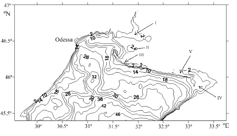
Fig.1. Bathymetry of the north-western shelf of the
I – the Dnieper-Bug estuary, II – Yagorlytsky, III – Tendrovsky,
IV – Karkinitsky and V – Dzharylgach bays
The system of model equations using the Boussinesq approximation, hydrostatic approximation and incompressibility of seawater in the Gromeko–Lamb form, the boundary conditions on the surface, at the bottom, on the solid lateral walls were written as follows [7, 8]. Note that a reduced sea level  was calculated from a discrete analog of the continuity equation taking into account the specification of the velocities at the open boundary of the domain [22].
In order to adapt the numerical model of the dynamics [7, 8] for the calculation of NWS circulation we made the following steps. Data array of the region bathymetry was processed, model parameters were chosen on the basis of preliminary experiments, river inflow locations and depths of estuaries were assigned, boundary conditions on the open boundaries of the region were selected and implemented, initial fields as well as fields of wind stress, heat flows, short-wave radiation, precipitation and evaporation were processed in order to be used in the model.
The numerical experiment 1 was carried out with resolution 500 m. The time step was equal to 10 s. The choice of values of horizontal and vertical turbulent viscosity coefficients was based on a series of specialized numerical experiments.
The numerical experiment 2 was carried out with resolution ~1.6 km. The time step was equal to 30 s.
Horizontal coefficients of turbulent viscosity and diffusion were equal to 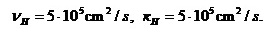
The total period of integration of model equations for the two experiments was 30 days (from October 14 to November 12 of 2007). Along the vertical, horizontal components of the current velocity were computed at 44 depths: 0.5; 1; 1.5; 2; 2.5; 3;…; 32; 34; 49 m.
Fields of currents, temperature and salinity, obtained from model for the entire sea on a 5 × 5 km horizontal grid within the Operative Oceanography project [23], were used to specify initial and the boundary conditions at the open boundary of the domain.
The u, v, T и S values, calculated at depths of 2.5, 5, 10, 15, 20, 25, 30 and 40 m, corresponding to the latitude of the liquid boundary, were linearly interpolated on the selected grids ( m и km) at each time instant.
In order to specify conditions on the open southern boundary we used the results of [22], where an efficiency of combined approach was shown on the basis of the simulation numerical experiments. The components of the current velocity, temperature, and salinity (the Dirichlet conditions) were specified in the boundary regions where water flowed into the domain (); conditions for u, v and radiation conditions for T and S were specified in the boundary regions where water flowed out of the domain ().
The vertical coefficients of turbulent exchange of momentum and diffusion were calculated according to the Philander–Pacanowski approximation [24] with , .
The fields of tangential wind stress, heat fluxes, short-wave irradiance fluxes, as well as precipitation and evaporation, obtained from data of the regional atmospheric model ALADIN and provided by the department of Marine Forecasts of MHI [23] and linearly interpolated to the selected grid, were specified for each day.
Used fields of wind stress were characterized by significant variability during the calculating period, wind velocity varied from values of 2.4 to 14.3 m/s .Northern, north-eastern, north-western and south-western winds with a maximum velocity 14.3 m/s (was recorded on October 16) dominated from 14 to 20 October, south-western winds with a maximum velocity 10.2 m/s (October 23) – from 21 to 25 October, northern winds with a maximum velocity 11.3 m/s (October 27) – from 26 to 28 October, western and south winds with a maximum velocity 7.1 m/s (October 29) – from October 29 to November 2, northern, north-eastern and western winds with a maximum velocity 11.3 m/s (November 5) – from 3 to 12 November.
We took into account the discharges of three rivers: Dnieper, Dniester, and
III. ANALYSIS of current fields of north-western shelf
The main direction of currents in the upper water layer changed from the south-west to the south, north, north-east, east, west and north-west. This was caused by changeable weather pattern that was observed during the calculating period.
Intense jets, directed to the south, were formed at depths of 10–26 m in case when currents in the upper water layer were directed to the south north, north-east and north-west. Intense jet currents, directed to the north, were observed at depths below 10 m in case of southern and south-eastern directions of currents dominated in the upper water layer. Fig. 2 shows current fields on October 29 (Fig. 2a) and November 3 (Fig. 2b), obtained in Experiment 1 at the depth of 10 m (every fifth arrow was drawn). We noted that trajectories of jets coincided with isobaths 19–28 m.
We compared the current fields obtained in Experiments 1 and 2 during the calculating period and found a qualitative correlation between the fields. The maximum values of currents, calculated in Experiment 1, were on average 5–10% higher than the values, obtained in Experiment 2.
Current fields of NWS had a complex mesoscale structure, characterized by eddies and jets. For the classification of obtained eddies we estimated a value of the local baroclinic deformation radius (Rd) for the selected coastal area of the
.jpg)
Fig. 2. Current fields (cm/c), calculated in Experiment 1: a – October 29 at the depth of 10 m;
b – November 3 at the depth of 10 m
As we know from [25], estimations of characteristic values of Rd for open areas of the
The baroclinic Rossby deformation radius was calculated using the formula:
Rd=[g(Δρ/ρ)H]0.5f -1,
where g – acceleration of gravity, Δρ – density gradient in the thermocline (~1.7*10-3 g/cm-3), ρ = 1 g/cm-3, Н – the upper layer thickness for October 2007 (~24 m) , f – Coriolis parameter corresponding to 46° N (~10-4 s-1). Rd was equal to ~6.4 km for the selected coastal zone. We assumed that mesoscale eddies had a radius bigger than local baroclinic Rossby deformation radius and Rossby number was much less than unity (R>Rd, Rо<1). We assumed that submesoscale eddies had a radius smaller than Rd and Rossby number was of the order of unity (R<Rd, Rо≈1).
Mesoscale еddies with a spatial scale of 8–12 km and a temporal scale of a few days were reproduced in the upper water layer near
Cyclonic eddy (R≈12 km >Rd, Rо≈0.18) was generated in the western part near the open boundary (Fig. 3a), anticyclonic eddies (Fig. 3b) were formed near
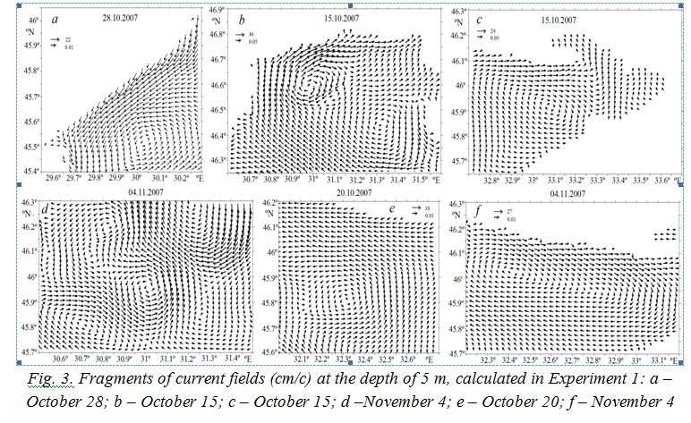
Fig. 3. Fragments of current fields (cm/c) at the depth of 5 m, calculated in Experiment 1: a – October 28; b – October 15; c – October 15; d –November 4; e – October 20; f – November 4
Mesoscale cyclonic eddy with a radius ~15 km, which was repeatedly registered in satellite observations, was generated in the period from 16 to 20 of October and from 1 to 5 of November, 2007 at depths of 1–24 m between the meridians 30.8° and 31.2° E. Fig. 4 shows the fields of surface currents on October 17 and 18 of 2007 calculated in Experiment 1 and 2 (every fifth and second arrow were drawn respectively).
.jpg)
Fig. 4. Current fields (cm/c) in the upper water layer on October 17 and 18, calculated
in Experiment 1 (a, d), Experiment 2 (b, e) and satellite images NOAA (c, f)
Intensification of currents inside the cyclonic eddy was observed in Experiment 1 on October 17 (Fig. 4a), and field structure was reproduced more accurately to the north of 46.4 °N compared with the results of Experiment 2 (Fig. 4b). This eddy wasn’t reproduced in Experiment 2 on October, 18 (Fig. 4e) in contrast to the results of Experiment 1 (Fig. 4d). Two anticyclonic eddies with a radius ~8 km were formed to the west and east of the cyclonic eddy. Correspondence between the results of Experiment 1 (Fig. 4a and Fig. 4d) and satellite observations on October, 17 and 18 of 2007 NOAA with resolution 1 km (Fig. 4c and Fig. 4f) was obtained. Formation of this eddy was a result of the influence of inhomogeneity of the bottom topography on the jet current. As it was noted in [26], cyclonic eddies were predominantly formed over submarine depressions.
We compared the current fields obtained in Experiments 1 and 2 during the calculating period and found a qualitative correlation between the fields, however, a number of eddies was absent and a field structure was smoother in the experiment with a lower resolution. Fig. 5 presents current fields obtained in experiments with a resolution of 500 m and ~1.6 km at depths of 5, 10 and 24 m on October 19, 2007 (every fifth and third arrow were drawn respectively, we marked on Fig. 5a, b, c elements of circulation that were absent on Fig. 5d, e, f)
.jpg)
Cyclonic eddy was reconstructed in the entire water layer in the eastern part of the region (between meridians 32.3º and 32.6º E) in Experiment 1. Cyclonic eddy in the central part of the area between meridians 30.8º and 31.2º E (Fig. 5a, b, c) was described above. It was observed in the entire water layer and its radius was ~12 km (Fig. 5a, b, c). Anticyclonic and cyclonic eddies with radius from ~4 to ~12 km in the central region at the depth of 5m (Fig. 5a), anticyclonic eddy with a radius ~10 km at the depth of 10 m in Karkinit bays (Fig. 5b), anticyclonic eddy with a radius of ~8 km at the depth of 24 m between the meridians 30.4 and 30.8º E (Fig. 5c) were reconstructed. These features were reproduced only in Experiment 1.
Fig. 6 shows fragments of current fields obtained in Experiment 1 on November 1, 4 and 10 of 2007 (Fig. 6a, b, c, every sixth arrow was drawn) and in Experiment 2 (Fig. 6d, e, f, every second arrow was drawn). We marked on Fig. 6a, b, c elements of circulation that were absent on Fig. 6d, e, f.
From the analysis of the current fields, calculated in experiments 1 and 2, we noted that due to the smaller grid size еddies with a radius of ~5 km between meridians 30.4º and 30.8º E on November 1 (Fig. 6a), cyclonic eddy with a radius of ~7 km between the meridians 31,9 and 32.1º E on November 4 (Fig. 6b), cyclonic eddies with a radius of ~12 km and anticyclonic eddy with a radius of ~5 km in the eastern part of the area on November 10 (Fig. 6c) were obtained .
Determining the type of small-scale eddies depends on the orbital velocity of an eddy. Analysis of the results of calculation of Rossby number Rо showed that values Rо≈1, as well as values Rо<1, have been obtained for the eddies with R<Rd during the calculating period.
.jpg)
IV. conclusions
Current fields of the north-western shelf of the
Due to the smaller grid size (500 m) meso- and submesoscale eddies have been obtained for the first time in the upper and deeper water layers of north-western shelf (anticyclonic and cyclonic eddies with a radius from ~4 to ~12 km in the central region, anticyclonic eddy with a radius of ~10 km in Karkinit bay, cyclonic eddies with a radius of ~12 km and anticyclonic eddy with a radius of ~5 km in the eastern part of the region).
These results convincingly confirm that a qualitative improvement in calculation accuracy of currents in the coastal zone requires the use of a few hundred meters of spatial resolution of numerical model.
This work was supported by the Russian Foundation for Basic Research (project no. 15–05–05423 А).
1. A.I. Androsovich, E.N. Mikhailova and N.B. Shapiro, “Numerical model and water circulation calculations in north-western part of the Black Sea,” Marine Hydrophysical Journal, vol. 5, pp. 28-42, 1994 (in Russian).
2. V.A. Ivanov, A.I. Kubryakov, E.N. Mikhailova and N.B. Shapiro, “Formation and evolution of eddies, caused by the river flow in the north-western shelf of the Black Sea,” Studies of the shelf zone of the Azov-Black Sea basin, pp. 147-167, 1995 (in Russian).
3. V.G. Alaev, Yu.N. Ryabtsev and N.B. Shapiro, “Adaptive calculation of current velocity on the shelf using a quasi-isopycnic model,” Marine Hydrophysical Journal, vol. 4, pp. 64-79, 1999 (in Russian).
4. D.V. Alekseev, V.A. Ivanov, E.V. Ivancha and L.V. Cherkesov, “Simulation of the evolution of wave fields on the north-western shelf of the Black Sea during a cyclone pas-sage,” Marine Hydrophysical Journal, vol. 1, pp. 42-54, 2005. (in Russian).
5. V.A. Ivanov, E.N. Mikhailova and N.B. Shapiro, “Simulation of wind upwelling on the north-western shelf of the Black Sea in the vicinity of the local features of the bottom relief, ” Marine Hydrophysical Journal, vol. 3, pp. 68-79, 2008. (in Russian).
6. S.G. Demyshev, V.A. Ivanov, N.V. Markova and L.V. Cherkesov, “Construction of the current fields in the Black Sea on the basis of eddy-resolving model with assimilation of climatic temperature and salinity fields,” Ecological safety of coastal and shelf areas and complex use of shelf resources, vol. 15, pp. 215-226, 2007. (in Russian).
7. S.G. Demyshev and G.K. Korotaev, “Numerical energy-balanced model of baroclinic currents of the ocean on the C-grid,” in Numerical models and results of calibration calculations of currents in the Atlantic Ocean, INM RAS, Moscow, 1992, pp. 163-231 (in Russian).
8. S.G. Demyshev, “A numerical model of online forecasting Black Sea currents,” Izvestiya Atmospheric and Oceanic Physics, vol. 48 (1), pp. 120-132, 2012.
9. I.F. Gertman, “The thermohaline structure of the sea water,” in Hydrometeorology and hydrochemistry seas of the USSR, vol. 4: Black Sea, Issue 1. Hydrometeorological conditions, S.Pb: Gidrometeoizdat, 1991, pp. 146-195 (in Russian).
10. S.N. Bulgakov and V.M. Kushnir, ”Features of current fields in the north-western part of the Black Sea,” Marine Hydrophysical Journal, vol. 5, pp. 66-78, 1996 (in Russian).
11. G.K. Korotaev, T. Oguz, A.A. Nikiforov, B.D. Beckley and C.J. Koblinsky, “Dy-namics of the Black Sea anticyclones derived from spacecraft remote sensing altimetry,” Earth Research from Space, vol. 6, pp. 1-10, 2002 (in Russian).
12. N.A. Diansky, V.B. Zalesny, S.N. Moshonkin and A.S. Rusakov, “High resolution modeling of the monsoon circulation in the Indian Ocean,” Oceanology, vol. 46 (6), pp. 608-628, 2006.
13. L.M. Ivanov, C.A. Collins, P. Marchesiello and T.M. Margolina, “On model valida-tion for meso/submesoscale currents: Metrics and application to ROMS off Central California,” Ocean Modelling, vol. 28 (4), pp. 209-225, 2009.
14. R.A. Ibrayev, R.N. Khabeev and K.V. Ushakov, “Eddy-resolving 1/10° model of the World Ocean,” Izvestiya Atmospheric and Oceanic Physics, vol. 48 (1), pp. 37-46, 2012.
15. L. Brannigan, D. Marshall, A. Naveira-Garabato and A. GeorgeNurser, “The seasonal cycle of submesoscale flows,” Ocean Modelling, vol. 92, pp. 69-84, 2015.
16. A.A. Rodionov, D.A. Romanenko, A.V. Zimin, I.E. Kozlov and B. Chapron, “Submezoscale structures of the White Sea waters and their dynamics. State and direction of the investigations,” Fundamental and Applied hydrophysics, vol. 7 (3), pp. 29-41, 2014 (in Russian).
17. V.G. Krivosheya, V.G. Yakubenko, A.Yu. Skirta and V.M. Shishkin, “Circulation and hydrological structure within the active layer of the 50-mile coastal part in the Russia sector of the Black Sea in August 2004,” Oceanology, vol. 47 (2), pp. 147-153, 2007.
18. A.G. Zatsepin, V.I. Baranov, A.A. Kondrashov, A.O. Korzh, V.V. Kremenetskiy et al., “Submesoscale eddies at the Caucasus Black Sea shelf and the mechanisms of their genera-tion,” Oceanology, vol. 51 (4), pp. 554-567, 2011.
19. G.F. Dzhiganshin and A.B. Polonsky, “Kinematic structure and mesoscale variability of the rim current near the coast of Crimea (according to the data of instrumental measurements in September 2008),” Marine Hydrophysical Journal, vol. 1, pp. 25-35, 2011 (in Russian).
20. S.S. Karimova, “Statistical analysis of the submesoscale eddies of the Baltic, Black and Caspian seas by satellite radar data,” Earth Research from Space, vol. 3, pp. 31-47, 2012. (in Russian).
21. B.V. Divinsky, S.B. Kuklev, A.G. Zatsepin and B.V. Chubarenko, “Simulation of submesoscale variability of currents in the Black Sea coastal zone,” Oceanology, vol. 55 (6), pp. 814-819, 2015.
22. S.G. Demyshev and N. A. Evstigneeva, “Numerical analysis of hydrophysical fields on the north-western shelf of the Black Sea,” Oceanology, vol. 53 (3), pp. 511-524, 2013.
23. Yu.B. Ratner, M.V. Martynov, T.M. Bayankina and S.V. Borodin, “Information flows in the real-time system of rapid monitoring of hydrophysical fields of the Black Sea and automation of their processing,” Environmental control systems, pp. 140-149, 2005 (in Russian).
24. R.C. Pacanowski and S.G.H. Philander, “Parameterization of vertical mixing in nu-merical models of tropical oceans,” J. Phys. Oceanogr., vol. 11 (11), pp. 1443-1451, 1981.
25. A.S. Blatov, N.P. Bulgakov and V.A. Ivanov, The variability of hydrophysical fields of the Black Sea, - Leningrad: Gidrometeoizdat, 1984, 240 p. (in Russian).
26. V.F. Kozlov and M.A. Sokolovskiy, “Stationary motion of a stratified fluid above a rough bottom,” Oceanology, vol. 18 (4), pp. 383-386, 1978.