


BISAC NAT010000 Ecology
BISAC NAT045050 Ecosystems & Habitats / Coastal Regions & Shorelines
BISAC NAT025000 Ecosystems & Habitats / Oceans & Seas
BISAC NAT045030 Ecosystems & Habitats / Polar Regions
BISAC SCI081000 Earth Sciences / Hydrology
BISAC SCI092000 Global Warming & Climate Change
BISAC SCI020000 Life Sciences / Ecology
BISAC SCI039000 Life Sciences / Marine Biology
BISAC SOC053000 Regional Studies
BISAC TEC060000 Marine & Naval
The work demonstrates the results of the 6-years complex ship-borne monitoring of coastal zone in the north-eastern part of the Black Sea, carried out by the Southern Branch of P.P.Shirshov Institute of Oceanology, RAS, on a marine cross-section at the Blue Bay (Gelendzhik) beam 1-2 times per month. Climatic changes and eutrophication exert a significant impact on the sea water at the coastal area. In case of the Black Sea these factors pile up with a permanent hydrogen sulphide contamination of the sea water below 80-200 meters depth (depending on the season and distance from the shore). Strong pycno-halocline at the depths from 70 to 160 meters, formed due to the inflow of high salinity water from the Marmara Sea, inhibits the mixing between the water layers and, as a result, also limits the oxygen transport into the deeper layers. The winter cooling reduces the pycno-halocline and enriches the top active layer, down to the cold intermediate layer (CIL), with oxygen and nutrients, which subsequently lead to a vernal phytoplankton bloom. Formation of the thermocline and upper quasi-homogeneous layer (UQL), caused by the water warming in spring, at large extent determines a thickness of phytoplankton-rich layer during the spring and summer seasons. The work demonstrates seasonal and interannual dynamics of the UQL, thermocline, CIL and hydrogen sulphide boundary position in the coastal zone of the north-eastern part of the Black Sea.
Black Sea, coastal zone, cold intermediate layer, upper quasi-homogeneous layer, thermocline, hydrogen sulphide boundary, monitoring.
I. Introduction
Complex monitoring of coastal ecosystem contributes a major part of the studies of the
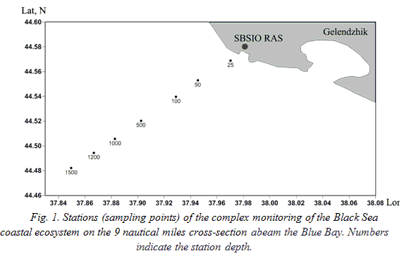
Since the monitoring cross-section ended with a 1500 meters depth station, and the distance between the neighboring stations was about 1.0-1.5 nautical miles, studied area had thoroughly covered both the shelf zone, affected by its own variability modes, and the continental slope, strongly influenced by the Black Sea Rim Current and mesoscale eddies.
The data, collected from the stations of the cross-section, allow us to study the intraseasonal, seasonal and interannual variability of key parameters of the
II. Materials and methods
Samples were gathered from the board of a small R/V “Ashamba”. The profiles of temperature, salinity and potential density were measured with the SBE 19plus CTD profiler on every station, from the surface to the bottom, or to the depth of 350 meters at the continental slope. The studies were performed with an average rate of once per two weeks during the following periods: from April 29 to December 7 (2010), from March 17 to December 14 (2011), from April 4 to November 26 (2012), from April 29 to November 5 (2013), from April 8 to November 28 (2014), from January 28 to December 11 (2015).
In total, 101 cruises of the small R/V “Ashamba” were performed, and more than 500 profiles of the above-mentioned hydrophysical parameters were acquired during the six-year period. Primary CTD data were filtered and vertically averaged at 1 meter intervals. Meteorological data of wind, air temperature, precipitation and surface water temperature and salinity were obtained from the Gelendzhik weather station.
III. Seasonal and interannual dynamics of the upper quasi-homogeneous layer (UQL) and main thermocline in the studied area in 2010-2015
Formation of the UQL begins in the end of April – beginning of May and is connected with the increase of air temperature and calm wind period, usually occurring in that time.
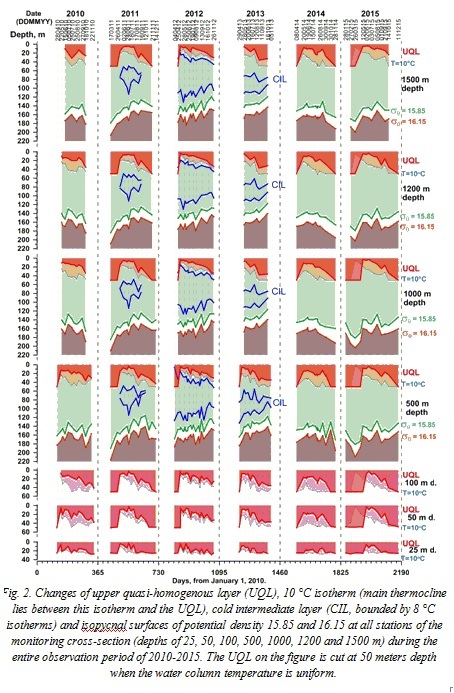
Conventionally, the temperature profile is used to determine the thickness of UQL. Its lower boundary, or bottom, is taken as a level where a sharp decrease of temperature (increase of its negative gradient amplitude) begins. A seasonal thermocline lies below, the isotherm of 10 °C assumed as its lower boundary. Fig. 2 shows the whole picture of the UQL and thermocline dynamics at all stations during the entire observation period. Structures of both the UQL and thermocline were similar at all stations, though the UQL was thicker at the stations closer to the shore (about 3.5-4 meters average difference between the station with 50 meters depth and the most remote station with 1500 meters depth). Average thickness of UQL during the warm season was about 20 meters. The thermocline, on the contrary, was somewhat more prolonged (about 2 m) at the deep stations with depths of 500-1500 meters. Average thickness of thermocline from May to October was about 14 meters.
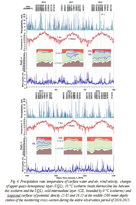
During all years of observation, the UQL warming reached its maximum in August (fig. 3), with a mean value of that maximum being about 26 °C and its peak values exceeding 28 °C. After that the cooling and concurrent deepening of UQL began. Mean temperature of UQL in October varied from 18 to 22 °C, depending on how cold was the autumn. Interannual dynamics of the UQL temperature was weak, and average annual temperature in the layer varied little, remaining in the interval of 21-23 °C. Coldest year in that point was 2011, while 2012 was the warmest. However, while temperature dynamics was insignificant, the UQL thickness from year to year changed far more (fig. 3), depending on precipitation rate, how warm was the spring and how developed was the cold intermediate layer (CIL).
The thermocline thickness increased during a year along with the UQL thickness, reaching maximum in July-August. After that, as the UQL cooled and thickened, it consecutively decreased and finally faded away in November (fig. 2, 3). During the years with a developed CIL, the thermocline thickness was almost half as much compared to the years when the CIL was not present. A joint analysis of temperature and salinity profiles was performed, and it has demonstrated that the spring halocline, as a rule, is forming along with the thermocline and on the same depth. However, in certain cases, which are observed in the coastal zone itself, the UQL has double-layered structure, characterized with a thin (2-4 meters thickness) subsurface highly freshened layer, possibly connected with the spread of river plumes. It was also found that a contribution of thermal stratification to the density stratification in the seasonal thermocline is almost always greater than the contribution of salinity stratification, and the ratio of the former to the latter increases from April to November.
.jpg)
The CIL, traditionally defined as a layer between 8 °C isotherms, is formed during winter, and its only source is the surface water (since the Bosporus inflow is warmer, about 12 °C). Variations in this layer determine a degree of penetration of surface water into the deeper layers and an extent of enrichment of the latter with oxygen and nutrients.
IV. Interannual and seasonal dynamics of the cold intermediate layer in the studied area during 2010-2015
Generally, the CIL in the north-eastern part of the
V. Position of isopycnic surfaces with potential density sq = 15.85 и 16.15 in the studied area during 2010-2015
Observations of hydrogen sulphide in the
Later it was repeatedly shown [3, 4] that depths of certain features of hydrochemical profiles (for example, extremums) in the central and peripheral Black Sea are locked to the particular density surfaces, i.e. there are no significant horizontal gradients of chemical variables along the same density surface. Thus one can estimate variability of certain chemical features in the depth field, including hydrogen sulphide boundary position, or the onset point, by using only CTD data. The hydrogen sulphide boundary is stable in the density field in the north-eastern
Depth of isopycnal surface of 15.85 in general determines a thickness of oxygenated layer, i.e. that part of water column, where basically life is able to exist. Below begins the suboxic part of the redox layer [6], where oxygen and H2S concentration are below the detection limit. Depth of isopycnal surface of 16.15 determines the depth of H2S appearance. Although the real depths of oxygen disappearance and H2S appearance may vary from the position of these isopycns, such fluctuations are relatively small and stretched in time in comparison with seasonal and local changes of water column in general.
The whole picture of depth variability of isopycnal surfaces of 15.85 and 16.15 during the studied years are shown on fig. 2.
Due to the winter ventilation, the depth of hydrogen sulphide boundary is usually maximal in the beginning of a year, and gradually, because of the continuous consumption of oxygen in the water column for organic matter oxidation, the H2S boundary rises up reaching its maximum in October. Such a picture we observed in 2011-2013 and, partly, in 2015. In 2010 and 2014, i.e. during the years when the CIL nominally was not observed, the H2S boundary rises up to its maximum in June-July, and then slowly goes down, reaching minimum in the end of September – October. The picture in 2015 in general conforms to the situation in the years with the CIL was presented. Although formally in 2015 a nominal CIL (T<8 °C) was not observed, values of the temperature minimum were close to the 8 °C boundary, occasionally decreasing below 8.1 °C. It is worth noticing that perhaps the CIL criterion should be reconsidered, and higher temperature accepted as the CIL boundary, but it is a subject for a separate study.
It was observed that the thickness of oxygenated layer (down to the isopycnal surface of 15.85) is on average greater during the years when the CIL is either not formed, or extremely strong. The latter can be explained that a massive CIL considerably enriches the deep layers with oxygen. And it seems that a weak oxygen ventilation during the “no CIL” years, on the one hand, does not supply a necessary oxygen saturation, but on the other hand, it also brings little amount of nutrients, thus limiting phytoplankton production and decreasing the amount of dead organic matter, which exhausts oxygen in the first place. During 2011 and 2013, when the CIL was weak (the CIL in 2013 was really the remnant from 2012), thickness of oxygenated layer was 10-15 meters less than in the other years.
Changes of hydrogen sulphide boundary position in the depth field can reach 60 meters during the year, and local fluctuations during 2-3 weeks – 30 meters.
Isopycnal surfaces of 15.85 и 16.15 followed each other variations, and the thickness of suboxic layer during the observation period changed little, from 15 to 25 meters. Monthly average depth of the isopycnal surface of 15.85 (thickness of oxygenated layer) is shown on fig. 3.
VI. Temperature of air and surface water (according to the Gelendzhik weather station) during 2010 to 2015
Measurements of temperature of air and surface water are performed by the Gelendzhik weather station every 3 hours. Fig. 4 shows changes of air temperature and surface sea water temperature for the entire observation period and corresponding changes in water column structure at the middle station of the cross-section (500 meters depth).
Minimum of monthly averaged temperatures of air and water was observed in February 2012: -0.3 °C and 6.6 °C for air and sea surface correspondingly. It should be noted that once the temperature of both air and water reached its maximum in August, temperature of sea surface was almost always greater than air temperature, up to the beginning of spring warming.
VII. Conclusions
The most noticeable part of the study is the interconnection of changes in all studied layers. Fluctuations of hydrogen sulphide boundary coincide with variations of CIL boundaries position, thermocline and UQL, demonstrating a close relation between all hydrophysical processes in the entire mass of water column. Therefore it is not correct to study the dynamics of the lower layers separately from the upper ones, and vice versa.
It is shown that variability of studied parameters in the depth field is high enough, and a situation can change a lot in just a short time. For example, in October 30, 2014, a large uprise of isopycnal surfaces of 15.85 and 16.15 was observed at the 500 meters depth station, caused, most likely, by a strong wind forcing. At the same day, due to a bad weather conditions, no sampling was performed on the stations with depth of 1000-1500 meters. As can be seen from the fig. 2, should there be no sampling on 500 meters depth station as well, we would assume a picture of a uniform decrease of H2S boundary as well as the suboxic layer, although we can be certain that, should the sampling at that stations had been performed, we would have observed the same uprise of the isopycnal surfaces. This fact demonstrates that when estimations of variability of hydrophysical parameters are based on a small amount of measurements, they will most likely lead to an inaccurate or even misleading result, and only a frequent monitoring can provide more or less proper picture of the processes that take place in the coastal area.
VIII. Acknowledgement
The monitoring studies were supported by the Russian Science Foundation, project No. 14-50-00095. Data processing and sample analyzing were supported by the Russian Foundation for Basic Research, project No. 14-05-00159.
1. J.W. Murray, H.W. Jannasch, S. Honjo, R.F. Anderson, W.S. Reeburgh, Z. Top, et al. “Unexpected changes in the oxic/anoxic interface in the Black Sea,” Nature, vol. 338, No. 6214. pp. 411-413, March 1989.
2. A.A. Bezborodov, “Variation of the boundary of anaerobic waters in the Black Sea as given by historical data,” in Complex Oceanographic Investigation of the Black Sea (in Russian). Ed. V.E. Zaika, 1990, Sevastopol: USSR Academy of Sciences, pp.76-114.
3. M.E. Vinogradov, Yu. P. Nalbandov, “Dependence of physical, chemical and biological parameters in pelagic ecosystem of the Black Sea upon the water density”, Oceanology, vol. 30 (5), pp. 769-777, October, 1990.
4. A.G. Rozanov, “Redox stratification of the Black Sea,” Oceanology, vol. 35(4), pp. 544-549, August, 1995.
5. E.V. Yakushev, V.K. Chasovnikov, J.W. Murray, S.V. Pakhomova, O.I. Podymov, P.A. Stunzhas, “Vertical hydrochemical structure of the Black Sea,” In: The Black Sea Environment. The Handbook of Environmental Chemistry, vol. 5Q, Ed. A.N. Kosarev, Berlin-Heidelberg: Springer-Verlag, 2008, pp. 277-307.
6. E.V. Yakushev, A. Newton, “Introduction: Redox Interfaces in Marine Waters,” In: Chemical Structure of Pelagic Redox Interfaces: Observation and Modeling. The Handbook of Environmental Chemistry, vol. 22, Ed. E.V. Yakushev. Heidelberg: Springer, 2013, pp. 1-12.